
How to Make a Line Graph in Google Sheets (2026 Guide)
 Carlos Garcia5/19/2026
If you've got time-series data in a Google Sheet — monthly revenue, weekly signups, daily active users, anything trending over time — a line graph is the cleanest way to visualize it. Google Sheets builds one in about 30 seconds, and the result is presentation-ready with a few quick customizations. This article walks through exactly how to make a line graph in Google Sheets in 2026, the customizations that take it from default to polished, and the practical tips for choosing line charts over the alternatives.
Free SEO + AI Search Audit. Line graphs show the trend of your data over time. The trend of your search visibility — across Google AND in ChatGPT, Claude, Perplexity, and Gemini — is just as worth tracking. Run your free audit → to see exactly where your site stands across every major search and AI platform in 60 seconds.
When Is a Line Graph the Right Chart?
In simple terms, line graphs are best for change over time when the X-axis represents a continuous timeline (days, weeks, months, quarters, years) and the Y-axis represents a measurable value (revenue, count, percentage, etc.). They beat column charts when:
- You have many time points (more than ~12)
- You're comparing multiple series and need a shared baseline
- The pattern matters more than the individual values
- You want to show the rate of change visually
For categorical comparisons (regions, products, departments) use a bar or column chart. For composition (parts of a whole) use a pie chart. For relationships between two variables, use scatter.
How to Make a Line Graph in Google Sheets (Step-by-Step)
Building a line graph takes about 30 seconds once your data is organized.
- Organize your data in two columns minimum. Column A: dates or time periods. Column B (and C, D, etc. for multi-series): numeric values. First row should be headers (e.g., "Month," "Revenue," "Expenses").
- Select the data range. Click and drag to highlight all cells including the header row.
- Go to Insert → Chart in the menu bar. Google Sheets inserts a chart and opens the Chart editor panel on the right.
- In the Setup tab, find the Chart type dropdown. By default, Google Sheets often picks a column chart. Change it to Line chart (or Smooth line chart for a curved version).
- Verify the data range, X-axis, and Series in the Setup tab. If Google Sheets guessed wrong about which column is the time axis, swap them here.
- Switch to the Customize tab to format the chart. Adjust title, colors, legend position, axis labels, and line thickness.
- Click outside the chart to deselect. The line graph is now embedded in your sheet.
That's it. To move or resize, click once and drag the corners. To return to the editor, double-click the chart.
Customizations That Make a Default Line Graph Presentation-Ready
A default Google Sheets line graph works. A few tweaks make it polished.
Chart Title and Axis Titles
In Customize → Chart & axis titles, write a specific title ("Q1-Q4 2026 Revenue Trend" beats "Revenue"). Add an X-axis title for the time period and a Y-axis title for the metric. Set font size to at least 14pt so the chart reads well in slides.
Line Color and Thickness
In Customize → Series, click each series to change its color individually. Use your brand colors for client reports, or pick semantic colors (green for revenue, red for costs, etc.) for performance dashboards. Increase line thickness from the default 2px to 3-4px for stronger visual presence.
Smooth Lines
In Customize → Series → Line smoothness, enable smoothing. The line gets a slight curve instead of sharp angles between data points. Makes time-series data feel more polished — especially with monthly or quarterly data where the individual points matter less than the trend.
Data Point Markers
Under Customize → Series → Point size, enable visible markers at each data point. Useful when you want viewers to be able to identify specific values. For very dense time-series data (daily data over a year), keep markers small or hide them to avoid clutter.
Legend Position
In Customize → Legend, set the legend to Bottom for charts with 3+ series and presentation use. For single-series charts, set the legend to None and rely on the chart title.
Y-Axis Number Formatting
In Customize → Vertical axis → Number format, format currency, percentages, or large numbers properly. Use `$#,##0` for currency, `0%` for percentages, or `#,##0` to add comma separators to large numbers. Default Google Sheets formatting often shows raw decimals — fix it.
Free SEO + AI Search Audit. Customizing a Google Sheets line graph is a small visual upgrade. Customizing what AI search engines see when they crawl your site is a much bigger one. Run a free audit of how your site performs in Google AND in ChatGPT, Claude, Perplexity, and Gemini — and where the biggest gaps are.
Gridlines
In Customize → Gridlines and ticks, reduce the major and minor gridline count. Default Google Sheets charts often have too many gridlines, which adds visual noise. Halving them improves readability without losing precision.
Trend Lines
For single-series line charts, you can overlay a trendline (linear, exponential, polynomial, or logarithmic) in Customize → Series → Trendline. Useful when the underlying pattern is more important than the individual data points.
How to Make a Multi-Series Line Graph
Multi-series line graphs are great for comparing related metrics over the same time period. Two examples: revenue vs expenses, or signups by acquisition channel.
- Lay out your data with the time period in Column A and each series in its own column (B, C, D, etc.).
- Select the entire range including all series columns.
- Insert → Chart, select Line chart.
- The Chart editor automatically treats each value column as a separate series with its own line and color.
- In Customize → Series, pick consistent colors and adjust line thickness for each.
For best readability, limit multi-series charts to 4-5 lines maximum. More than that and the chart becomes spaghetti — split into multiple charts or use a different visualization.
Common Mistakes to Avoid
A few line-graph mistakes that show up constantly:
1. Using a Line Chart for Non-Continuous Data
Line charts imply continuity between data points. If your X-axis is categories (regions, products), use a bar chart instead. Lines between unrelated categories suggest a relationship that doesn't exist.
2. Truncated Y-Axis That Exaggerates Changes
Default line graphs often start the Y-axis at a value higher than zero. This makes small changes look dramatic. For honest charts, start the Y-axis at zero unless there's a specific reason not to. In Customize → Vertical axis, set the Min value to 0.
3. Too Many Series
Five lines on one chart is the practical maximum. Beyond that, viewers can't track individual lines. Split into multiple charts grouped by category, or use a single line plus a separate detail table.
4. Missing or Misleading Axis Labels
A line chart without an X-axis title leaves viewers guessing about time periods. A Y-axis without units leaves them guessing whether 50 means dollars, thousands, percentage, or something else. Always label both axes.
Free SEO + AI Search Audit. Avoiding mistakes in your charts is one part of clear communication. Avoiding blind spots in your search performance is another. Get a free audit of how your site performs across Google AND every major AI search platform.
When Should You Use a Line Graph vs an Alternative?
Line graphs are great for continuous data — but not the only option.
Use a Line Graph When...
You're showing change over time with continuous data points. Trends matter more than individual values. Multiple series share a common baseline.
Use a Column Chart Instead When...
The time periods are discrete and you want to emphasize individual values (monthly revenue with 12 months you want to compare exactly). Column charts also work better for showing year-over-year comparisons side by side.
Use an Area Chart Instead When...
You want to emphasize cumulative volume rather than the line itself. Useful for stacked area charts showing how different segments contribute to a total over time.
Use a Scatter Plot Instead When...
The X-axis isn't a continuous timeline but a numeric variable (like ad spend or price). Scatter plots make the relationship between two variables clearer than a line graph would.
Limitations of Google Sheets Line Graphs
Limited visual sophistication. For polished executive dashboards, Looker Studio and Tableau offer more customization (custom themes, annotations, interactive features).
No native annotations. Marking a specific event on the line (a product launch, a marketing campaign start) requires manual workarounds or drawn shapes.
Performance on large datasets degrades. Line charts on 10,000+ data points slow down the sheet. For really dense time-series data, aggregate or sample first.
Limited interactivity. Sheets line graphs don't support filtering, drill-down, or tooltip customization the way BI tools do.
Mobile editing is awkward. Creating or modifying a line graph on a phone is painful. Edit on desktop.
Final Thoughts
A line graph in Google Sheets is the fastest way to turn time-series data into a visual story. For business communication, internal dashboards, and quick analyses, it's the right tool — and the 30-second build time is unbeatable. For more polished or interactive work, graduate to Looker Studio or Tableau.
Once your charts are clean, the bigger question is whether your business is reaching the right people in the first place. In 2026, that increasingly means showing up not just in Google but in ChatGPT, Claude, Perplexity, and Gemini when buyers ask AI for product recommendations. Most teams have no idea where they stand in those AI answers. Run a free audit to see exactly where your site performs across Google AND every major AI search platform — and which fixes will move your traffic the fastest this quarter.