How to Click the Chart Legend in Excel (2026 Guide)

If you've been trying to click a chart legend in Excel to format it, move it, or hide a series — and the click either does nothing or does the wrong thing — you're not alone. Excel's chart legend has surprisingly nuanced click behavior: a single click selects the whole legend, a second click selects a specific entry, a right-click opens a context menu, and double-clicking opens the format pane. Clicking a chart legend in Excel lets you select, format, move, resize, or filter series by entry, but the exact result depends on whether you single-click, double-click, or right-click, and how many times you've already clicked. This guide walks through every click interaction, what each does, common reasons clicks don't work, and how to use the legend as a filter.

Free SEO + AI Search Audit. Excel chart interactions are subtle once you know them. SEO + AI search visibility is the same — small details matter. A free SEO + AI search audit shows you exactly where you stand across Google AND in AI search engines like ChatGPT, Claude, Perplexity, and Gemini. Run your free audit → to see where your site stands in 60 seconds.

How to Click the Chart Legend in Excel: The Direct Answer

In simple terms, clicking a chart legend in Excel always begins with a single left-click on the legend area, which selects the entire legend; subsequent actions (formatting, moving, resizing, filtering, deleting) depend on what you do next. The legend is a separate chart element with its own selection state, format pane, and context menu.

Common interactions:

• Single left-click on the legend area → selects the whole legend
• Single left-click on a specific entry (after the legend is selected) → selects that one entry only
• Double-click on the legend → opens the Format Legend task pane
• Right-click on the legend → opens a context menu with formatting and delete options
• Drag the legend → moves it within the chart area
• Click a sizing handle → resizes the legend
• Click in the legend after selecting the chart filter funnel → toggles series visibility

Step-by-Step: Selecting the Chart Legend

The first click sets up everything else.

Step 1: Click the Chart Background

Click anywhere inside the chart frame (but not on a data point, axis, or title). This activates the chart's editing mode and shows chart-element handles.

Step 2: Click the Legend Area

Click directly on the legend box (the area with colored markers and series names). You'll see a rectangular selection border with eight handles around the legend.

Step 3: Confirm the Legend Is Selected

Look at the chart Format tab in the ribbon. The dropdown at the far left should now say "Legend." That confirms you have the legend selected, not the entire chart.

How to Format the Legend by Clicking

Once selected, you have multiple ways to format it.

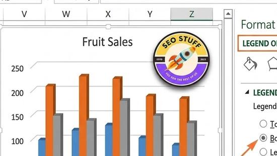
Method 1: Double-Click to Open the Format Pane

Double-click anywhere on the legend area. The Format Legend task pane opens on the right side of Excel. You can change position, fill, border, font, and effects.

Method 2: Right-Click for Quick Format Options

Right-click the legend to open the context menu. Options include Format Legend..., Font..., Delete, and Add Data Labels.

Method 3: Use the Chart Format Ribbon

With the legend selected, go to Chart Design → Add Chart Element → Legend to change its position (top, right, left, bottom, none). Or go to Format → Format Selection for the same task pane as the double-click method.

Method 4: Use the + Chart Elements Button

Click the chart, then click the + icon next to the chart's top-right corner. Hover Legend and click the right-arrow for position options.

How to Click a Specific Legend Entry

Single-clicking a legend selects the whole legend. To click a single entry:

Step 1: First, Select the Legend

Single-click the legend area as in the steps above. You'll see the whole-legend selection border.

Step 2: Click the Specific Entry

Click directly on the colored marker or the text of a single legend entry. The whole-legend border becomes a smaller selection just around that one entry.

Step 3: Confirm the Entry-Level Selection

The Format ribbon dropdown should now say "Legend Entry 1" (or whichever index). You can now format just that entry — font color, font weight, etc.

Step 4: Use Format Selection

Click Format → Format Selection to open a Format Legend Entry pane with options specific to that entry.

How to Move the Chart Legend by Clicking and Dragging

The legend isn't locked to its default position.

Step 1: Click to Select

Single-click the legend area.

Step 2: Hover Over the Edge

Move the cursor to the edge of the legend (not the resize handles). The cursor should change to a four-arrow move icon.

Step 3: Click and Drag

Click and hold, then drag the legend to a new position inside the chart area.

Step 4: Release

Release the mouse. The legend stays at the new position.

Note: dragging the legend overlays it on the chart's plot area; the chart automatically resizes the plot area to fit the legend's docked position only when you use Chart Design → Add Chart Element → Legend → [position].

How to Resize the Chart Legend

Resizing changes the legend's bounding box.

Step 1: Click to Select

Single-click the legend.

Step 2: Hover Over a Corner or Edge Handle

The eight selection handles let you resize from any side or corner. Hover over a handle to get the resize cursor.

Step 3: Click and Drag

Drag to resize. The legend's text wraps or condenses based on the new dimensions.

Free SEO + AI Search Audit. Excel chart legends require precise clicks. A free SEO + AI search audit requires zero clicks — just enter your URL. Get a free audit of how your site performs across Google AND every major AI search platform.

How to Use the Legend as a Filter (Show/Hide Series)

A clicked-but-checked-on legend entry shows the series; unchecked hides it. This filtering happens through the chart Filter funnel, not direct legend clicks.

Step 1: Click the Chart's Funnel Icon

In Excel, click the chart, then click the funnel icon at the top-right corner (next to + and paint icons).

Step 2: Uncheck a Series

In the panel that opens, uncheck a series name. The chart updates to hide that series; the legend entry disappears from the legend.

Step 3: Re-check to Show

Re-check the series to bring it back.

Note: in some Excel versions, clicking a legend entry directly toggles series visibility in addition to the funnel approach. Behavior varies by version.

How to Delete the Chart Legend

Method 1: Right-Click → Delete

Right-click the legend → Delete.

Method 2: Press Delete Key

Click the legend, then press Delete on the keyboard.

Method 3: Toggle Off in Chart Elements

Click the + Chart Elements icon next to the chart → uncheck Legend.

Common Reasons Clicking the Legend Doesn't Work

A few patterns that confuse people.

1. You're Clicking Outside the Legend Bounding Box

The legend has a specific clickable area. If your click lands just outside (in the chart's empty space), Excel selects the chart background instead.

2. The Chart Is Locked or Protected

If the worksheet is protected with "Edit objects" disabled, you can't interact with chart elements. Review → Unprotect Sheet to fix.

3. The Chart Is Embedded in a Pivot Chart Filter Pane

Pivot charts have filter buttons that look similar to legend entries but behave differently. The actual legend (if present) is a separate element.

4. You're in Read-Only Mode

If Excel opened the file as read-only (yellow bar at the top), you can view the chart but can't modify the legend. Click Edit Anyway in the yellow bar.

5. Mobile/Tablet Touch Interactions

On touch devices, tap behavior may differ from mouse clicks. A first tap may select the chart, requiring a second tap on the legend, and a third on a specific entry.

6. Hidden Chart Layer in PowerPoint or Word

If you're working with an Excel chart embedded in PowerPoint or Word, clicks may select the wrapper object rather than the chart. Double-click the chart to enter Excel edit mode first.

Keyboard Shortcuts for the Chart Legend

A few keyboard shortcuts speed things up.

Tab — cycles through chart elements when the chart is selected (legend is one of the cycle stops)

Arrow keys — when a legend entry is selected, arrow keys move between entries

Enter or F2 — opens the Format pane for the selected element

Delete — removes the selected element

Esc — deselects the current chart element

Chart Legend Click Behavior vs Other Chart Elements

How the legend compares.

Legend

Single-click selects the whole legend, second click selects a single entry, double-click opens format pane

Axis

Single-click selects the axis, double-click opens Format Axis pane

Data Series

Single-click selects the whole series, second click selects a single data point

Chart Title

Single-click selects the title box, second click enters text-editing mode

Plot Area

Single-click selects the plot area background; useful for changing the background color

Free SEO + AI Search Audit. Mastering Excel chart legend clicks is a small productivity win. Knowing where your site shows up in AI search is a much bigger one. Run a free audit of how your site performs across Google AND every major AI search platform.

Limitations of Chart Legend Clicking in Excel

A few honest constraints.

Behavior varies across Excel versions. Excel 2016, 2019, 2021, 2024, Microsoft 365, and the Web app all have slightly different click behaviors. Direct legend-click-to-filter is more common on newer versions.

Touch devices have inconsistent click handling. Tap-and-hold may register as right-click but often doesn't. Mouse input is more reliable for legend interactions.

Excel for the Web has fewer right-click options. Right-click context menus in the browser version are reduced. Use the Format pane via the chart formatting sidebar instead.

Locked charts can't be clicked. Workbook protection can disable chart-element interactions entirely.

Pivot chart filter buttons look similar to legend entries. Mistakenly clicking a pivot chart filter button instead of a legend entry is a common confusion point.

Final Thoughts

Clicking the chart legend in Excel is straightforward once you understand the multi-click pattern: first click selects the whole legend, second click drills into a single entry, double-click opens the format pane, and right-click gives you the context menu. Drag to move, handle-drag to resize, Delete to remove, and the filter funnel toggles series visibility. The only gotchas are protected workbooks, read-only mode, and the slight version-to-version variability in direct-legend-click filtering behavior. Once you internalize the click hierarchy, formatting and adjusting chart legends becomes a five-second task instead of a frustrating one.

Beyond Excel productivity, the bigger 2026 question for most marketing teams is whether your content is even being found. Increasingly, buyers use AI search engines like ChatGPT, Claude, Perplexity, and Gemini for product recommendations — and most teams have zero measurement of how they show up there. While you're cleaning up chart formatting in your Excel reports, you may be invisible in the AI answers shaping more and more buying decisions. Run a free audit to see exactly where your site performs across Google AND every major AI search platform — and which fixes will move your traffic the fastest this quarter.